
Transforms
Data does not always come in its final processed form that is required for training machine learning algorithms. We use transforms to perform some manipulation of the data and make it suitable for training.
All TorchVision datasets have two parameters -
transformto modify the features andtarget_transformto modify the labels - that accept callables containing the transformation logic. The torchvision.transforms module offers several commonly-used transforms out of the box.The FashionMNIST features are in PIL Image format, and the labels are integers. For training, we need the features as normalized tensors, and the labels as one-hot encoded tensors. To make these transformations, we use
ToTensorandLambda.我们从磁盘读取图片和标签,这些图片和标签无法直接喂入神经网路中,传入照片以后,会通过Transforme对图片做一些约束和一些变换,使其满足神经网络所需要输入的要求。一般在
DataSet中定义,在getItem中应用。target_transform也是一样的,假设我们的标签读取的是整型的,但我们希望神经网络的输出是一个
one-hot的形式以更方便的计算交叉熵,这个时候,就将从磁盘中读取的整型标签进行一个变换,变为one-hot编码的格式。
Build the Neural Network
Neural networks comprise of layers/modules that perform operations on data. The torch.nn namespace provides all the building blocks you need to build your own neural network. Every module in PyTorch subclasses the nn.Module. A neural network is a module itself that consists of other modules (layers). This nested structure allows for building and managing complex architectures easily.
import os
import torch
from torch import nn
from torch.utils.data import DataLoader
from torchvision import datasets, transforms
Get Device for Training
We want to be able to train our model on a hardware accelerator like the GPU or MPS, if available. Let’s check to see if torch.cuda or torch.backends.mps are available, otherwise we use the CPU.
device = (
    "cuda"
    if torch.cuda.is_available()
    else "mps"
    if torch.backends.mps.is_available()
    else "cpu"
)  # 判断我们当前的环境,能否使用Cuda,可用,则将model、parameter放在GPU上,如果不可用,则放在CPU上运行。
print(f"Using {device} device")
Define the Class
We define our neural network by subclassingnn.Module, and initialize the neural network layers in__init__. Everynn.Modulesubclass implements the operations on input data in theforwardmethod.
class NeuralNetwork(nn.Module):  # 所有的网络都要继承nn.Module父类,继承关系,一般要实现__init__方法和forward方法
    def __init__(self):  # 创建子模块
        super().__init__()  # 首先调用父类的init方法
        self.flatten = nn.Flatten()  # 创建第一个模块Flatten层
        self.linear_relu_stack = nn.Sequential(  # 创建第二个线性激活堆叠模块,nn.Sequential()会将其中的层串联
            nn.Linear(28*28, 512),  # ~MLP,第一个参数为输入的特征维度,第二餐参数为隐含层的大小
            nn.ReLU(),  # 激活函数https://baike.baidu.com/item/ReLU%20%E5%87%BD%E6%95%B0/22689567?fr=ge_ala
            nn.Linear(512, 512),
            nn.ReLU(),
            nn.Linear(512, 10),  # 最后一层10,分类,logits,将其放入softmax得到每一个类别的概率
        )

    # 定义了model的一个前向运算逻辑
    def forward(self, x):  # 通常不需要显式调用,实例化NeuralNetwork对象后,直接NeuralNetwork(x)就默认调用此方法
        x = self.flatten(x)  # 先对x的维度铺平
        logits = self.linear_relu_stack(x)  # 再放入linear_relu_stack
        return logits
We create an instance of NeuralNetwork, and move it to the device, and print its structure.
model = NeuralNetwork().to(device)  # 实例化,调用module的to函数,这边是将该网络的全部都放入device设备运行
print(model)  # 能看到model的每个子模块,和其输入输出的大小
'''
NeuralNetwork(
  (flatten): Flatten(start_dim=1, end_dim=-1)
  (linear_relu_stack): Sequential(
    (0): Linear(in_features=784, out_features=512, bias=True)
    (1): ReLU()
    (2): Linear(in_features=512, out_features=512, bias=True)
    (3): ReLU()
    (4): Linear(in_features=512, out_features=10, bias=True)
  )
)
'''
若想查看每一层的参数数目(可训练+不可训练)
sksq96/pytorch-summary: Model summary in PyTorch similar to model.summary() in Keras (github.com)
import torch
import torch.nn as nn
import torch.nn.functional as F
from torchsummary import summary

class Net(nn.Module):
    def __init__(self):
        super(Net, self).__init__()
        self.conv1 = nn.Conv2d(1, 10, kernel_size=5)
        self.conv2 = nn.Conv2d(10, 20, kernel_size=5)
        self.conv2_drop = nn.Dropout2d()
        self.fc1 = nn.Linear(320, 50)
        self.fc2 = nn.Linear(50, 10)

    def forward(self, x):
        x = F.relu(F.max_pool2d(self.conv1(x), 2))
        x = F.relu(F.max_pool2d(self.conv2_drop(self.conv2(x)), 2))
        x = x.view(-1, 320)
        x = F.relu(self.fc1(x))
        x = F.dropout(x, training=self.training)
        x = self.fc2(x)
        return F.log_softmax(x, dim=1)

device = torch.device("cuda" if torch.cuda.is_available() else "cpu") # PyTorch v0.4.0
model = Net().to(device)

summary(model, (1, 28, 28))
# 给出每一层的名称,和参数数目
----------------------------------------------------------------
Layer (type) Output Shape Param #
================================================================
Conv2d-1 [-1, 10, 24, 24] 260
Conv2d-2 [-1, 20, 8, 8] 5,020
Dropout2d-3 [-1, 20, 8, 8] 0
Linear-4 [-1, 50] 16,050
Linear-5 [-1, 10] 510
================================================================
Total params: 21,840
Trainable params: 21,840
Non-trainable params: 0
----------------------------------------------------------------
Input size (MB): 0.00
Forward/backward pass size (MB): 0.06
Params size (MB): 0.08
Estimated Total Size (MB): 0.15
----------------------------------------------------------------To use the model, we pass it the input data. This executes the model’s
forward, along with some background operations. Do not callmodel.forward()directly!Calling the model on the input returns a 2-dimensional tensor with dim=0 corresponding to each output of 10 raw predicted values for each class, and dim=1 corresponding to the individual values of each output. We get the prediction probabilities by passing it through an instance of the
nn.Softmaxmodule.
X = torch.rand(1, 28, 28, device=device)
logits = model(X)
pred_probab = nn.Softmax(dim=1)(logits)  # 对第一个维度计算softmax归一化
y_pred = pred_probab.argmax(1)  # 取最大概率得到样本类别
print(f"Predicted class: {y_pred}")
'''
Predicted class: tensor([7], device='cuda:0')
'''
Model Layers
Let’s break down the layers in the FashionMNIST model. To illustrate it, we will take a sample minibatch of 3 images of size 28x28 and see what happens to it as we pass it through the network.
input_image = torch.rand(3,28,28)
print(input_image.size())
'''
torch.Size([3, 28, 28])
'''
nn.Flatten
We initialize the nn.Flatten layer to convert each 2D 28x28 image into a contiguous array of 784 pixel values ( the minibatch dimension (at dim=0) is maintained).
flatten = nn.Flatten()
flat_image = flatten(input_image)  # 第一维到最后一维,全部铺平为一个维度,最后仅保留[batch_size, other]
print(flat_image.size())
'''
torch.Size([3, 784])
'''CLASStorch.nn.Flatten(start_dim=1, end_dim=-1)[SOURCE]
- start_dim (int) – first dim to flatten (default = 1).
- end_dim (int) – last dim to flatten (default = -1).
Examples::
input = torch.randn(32, 1, 5, 5)
# With default parameters
m = nn.Flatten()
output = m(input)
output.size()
# With non-default parameters
m = nn.Flatten(0, 2)
output = m(input)
output.size()
nn.Linear
The linear layer is a module that applies a linear transformation on the input using its stored weights and biases.
layer1 = nn.Linear(in_features=28*28, out_features=20)  # input.size[3, 784] => [28*28, 20]
hidden1 = layer1(flat_image)
print(hidden1.size())
'''
torch.Size([3, 20])
'''CLASStorch.nn.Linear(in_features, out_features, bias=True, device=None, dtype=None)[SOURCE]
Parameters
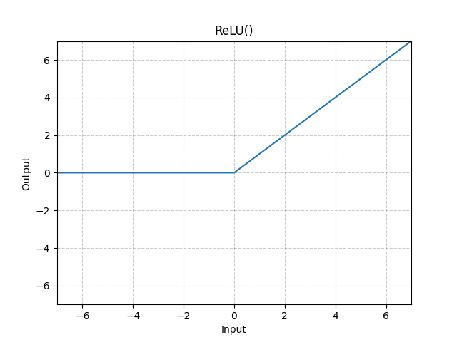
nn.ReLU
Non-linear activations are what create the complex mappings between the model’s inputs and outputs. They are applied after linear transformations to introduce nonlinearity, helping neural networks learn a wide variety of phenomena.
In this model, we use nn.ReLU between our linear layers, but there’s other activations to introduce non-linearity in your model.(非线性激活,增强模型的表达能力)
print(f"Before ReLU: {hidden1}\n\n")
hidden1 = nn.ReLU()(hidden1)
print(f"After ReLU: {hidden1}")
'''
Before ReLU: tensor([[ 0.4158, -0.0130, -0.1144,  0.3960,  0.1476, -0.0690, -0.0269,  0.2690,
          0.1353,  0.1975,  0.4484,  0.0753,  0.4455,  0.5321, -0.1692,  0.4504,
          0.2476, -0.1787, -0.2754,  0.2462],
        [ 0.2326,  0.0623, -0.2984,  0.2878,  0.2767, -0.5434, -0.5051,  0.4339,
          0.0302,  0.1634,  0.5649, -0.0055,  0.2025,  0.4473, -0.2333,  0.6611,
          0.1883, -0.1250,  0.0820,  0.2778],
        [ 0.3325,  0.2654,  0.1091,  0.0651,  0.3425, -0.3880, -0.0152,  0.2298,
          0.3872,  0.0342,  0.8503,  0.0937,  0.1796,  0.5007, -0.1897,  0.4030,
          0.1189, -0.3237,  0.2048,  0.4343]], grad_fn=<AddmmBackward0>)
# 激活之前包含负数,激活之后过滤掉负数
After ReLU: tensor([[0.4158, 0.0000, 0.0000, 0.3960, 0.1476, 0.0000, 0.0000, 0.2690, 0.1353,
         0.1975, 0.4484, 0.0753, 0.4455, 0.5321, 0.0000, 0.4504, 0.2476, 0.0000,
         0.0000, 0.2462],
        [0.2326, 0.0623, 0.0000, 0.2878, 0.2767, 0.0000, 0.0000, 0.4339, 0.0302,
         0.1634, 0.5649, 0.0000, 0.2025, 0.4473, 0.0000, 0.6611, 0.1883, 0.0000,
         0.0820, 0.2778],
        [0.3325, 0.2654, 0.1091, 0.0651, 0.3425, 0.0000, 0.0000, 0.2298, 0.3872,
         0.0342, 0.8503, 0.0937, 0.1796, 0.5007, 0.0000, 0.4030, 0.1189, 0.0000,
         0.2048, 0.4343]], grad_fn=<ReluBackward0>)
'''CLASStorch.nn.ReLU(inplace=False)[SOURCE]
Parameters
inplace (bool) – can optionally do the operation in-place. Default:
FalseShape:
- Input: (∗)(∗), where ∗∗ means any number of dimensions.
- Output: (∗)(∗), same shape as the input.
nn.Sequential
nn.Sequential is an ordered container of modules. (关于模块的一个有序的容器)The data is passed through all the modules in the same order as defined. You can use sequential containers to put together a quick network like seq_modules.(当我们把一些model作为Sequential的实例化参数后,这些数据就会有序的经过这些模块,最终算出一个结果)seq_modules = nn.Sequential(
flatten,
layer1,
nn.ReLU(),
nn.Linear(20, 10)
)
input_image = torch.rand(3,28,28)
logits = seq_modules(input_image)CLASStorch.nn.Sequential(args: Module)[SOURCE]*
A sequential container.
Modules will be added to it in the order they are passed in the constructor. Alternatively, an
OrderedDictof modules can be passed in. Theforward()method ofSequentialaccepts any input and forwards it to the first module it contains. It then “chains” outputs to inputs sequentially for each subsequent module, finally returning the output of the last module.The value a
Sequentialprovides over manually calling a sequence of modules is that it allows treating the whole container as a single module, such that performing a transformation on theSequentialapplies to each of the modules it stores (which are each a registered submodule of theSequential).What’s the difference between a
Sequentialand atorch.nn.ModuleList? AModuleListis exactly what it sounds like–a list for storingModules! On the other hand, the layers in aSequentialare connected in a cascading way.Example:
# Using Sequential to create a small model. When `model` is run,
# input will first be passed to `Conv2d(1,20,5)`. The output of
# `Conv2d(1,20,5)` will be used as the input to the first
# `ReLU`; the output of the first `ReLU` will become the input
# for `Conv2d(20,64,5)`. Finally, the output of
# `Conv2d(20,64,5)` will be used as input to the second `ReLU`
model = nn.Sequential(
          nn.Conv2d(1,20,5),
          nn.ReLU(),
          nn.Conv2d(20,64,5),
          nn.ReLU()
        )

# Using Sequential with OrderedDict. This is functionally the
# same as the above code
model = nn.Sequential(OrderedDict([
          ('conv1', nn.Conv2d(1,20,5)),
          ('relu1', nn.ReLU()),
          ('conv2', nn.Conv2d(20,64,5)),
          ('relu2', nn.ReLU())
        ]))
nn.Softmax
The last linear layer of the neural network returns logits - raw values in [-infty, infty] - which are passed to the nn.Softmax module. The logits are scaled to values [0, 1] representing the model’s predicted probabilities for each class. dim parameter indicates the dimension along which the values must sum to 1.softmax = nn.Softmax(dim=1)
pred_probab = softmax(logits)CLASStorch.nn.Softmax(dim=None)[SOURCE](仅对某一维度进行softmax)
Shape:
- Input: (∗)(∗) where * means, any number of additional dimensions
- Output: (∗)(∗), same shape as the input
Returns
a Tensor of the same dimension and shape as the input with values in the range [0, 1]
Parameters
dim (int) – A dimension along which Softmax will be computed (so every slice along dim will sum to 1).
Return type
None
Examples:
>>> m = nn.Softmax(dim=1)
>>> input = torch.randn(2, 3)
>>> output = m(input)  # 关于input第一维归一化的结果
Model Parameters
Many layers inside a neural network are parameterized, i.e. have associated weights and biases that are optimized during training. Subclassing
nn.Moduleautomatically tracks all fields defined inside your model object, and makes all parameters accessible using your model’sparameters()ornamed_parameters()methods.In this example, we iterate over each parameter, and print its size and a preview of its values.
print(f"Model structure: {model}\n\n")

for name, param in model.named_parameters():
    print(f"Layer: {name} | Size: {param.size()} | Values : {param[:2]} \n")
'''
Model structure: NeuralNetwork(
  (flatten): Flatten(start_dim=1, end_dim=-1)
  (linear_relu_stack): Sequential(
    (0): Linear(in_features=784, out_features=512, bias=True)
    (1): ReLU()
    (2): Linear(in_features=512, out_features=512, bias=True)
    (3): ReLU()
    (4): Linear(in_features=512, out_features=10, bias=True)
  )
)
# 1和3是relu层,没有参数,所以未打印
0 nn.Linear(28*28, 512),
Layer: linear_relu_stack.0.weight | Size: torch.Size([512, 784]) | Values : tensor([[ 0.0273,  0.0296, -0.0084,  ..., -0.0142,  0.0093,  0.0135],
        [-0.0188, -0.0354,  0.0187,  ..., -0.0106, -0.0001,  0.0115]],
       device='cuda:0', grad_fn=<SliceBackward0>)

Layer: linear_relu_stack.0.bias | Size: torch.Size([512]) | Values : tensor([-0.0155, -0.0327], device='cuda:0', grad_fn=<SliceBackward0>)
2 nn.Linear(512, 512),
Layer: linear_relu_stack.2.weight | Size: torch.Size([512, 512]) | Values : tensor([[ 0.0116,  0.0293, -0.0280,  ...,  0.0334, -0.0078,  0.0298],
        [ 0.0095,  0.0038,  0.0009,  ..., -0.0365, -0.0011, -0.0221]],
       device='cuda:0', grad_fn=<SliceBackward0>)

Layer: linear_relu_stack.2.bias | Size: torch.Size([512]) | Values : tensor([ 0.0148, -0.0256], device='cuda:0', grad_fn=<SliceBackward0>)
4 nn.Linear(512, 10),
Layer: linear_relu_stack.4.weight | Size: torch.Size([10, 512]) | Values : tensor([[-0.0147, -0.0229,  0.0180,  ..., -0.0013,  0.0177,  0.0070],
        [-0.0202, -0.0417, -0.0279,  ..., -0.0441,  0.0185, -0.0268]],
       device='cuda:0', grad_fn=<SliceBackward0>)

Layer: linear_relu_stack.4.bias | Size: torch.Size([10]) | Values : tensor([ 0.0070, -0.0411], device='cuda:0', grad_fn=<SliceBackward0>)
'''
还不快抢沙发